# Addition
1 + 2 + 3 + 4 + 5
[1] 15In this chapter, we introduce the fundamental building blocks of R: objects and functions. In R, everything is an object — including data, datasets, and even functions themselves. Functions perform actions on other objects, making them essential tools for working with data. We begin by exploring the concept of an object, along with the different data types and data structures that R works with. Furthermore, we explain functions in more detail, discuss some of the main functions of base R, and see how we can create our own functions.
Let’s start with a very simple arithmetic example. In the code below we employ addition, subtraction, multiplication, division, exponentiation and modulo (remainder of a division).
# Addition
1 + 2 + 3 + 4 + 5[1] 15# Subtraction
10 - 5[1] 5# Multiplication
2 * 3[1] 6# Division
5 / 4[1] 1.25# Exponentiation
2 ^ 4[1] 16# Remainder
5 %% 4[1] 1As explained in the Introduction to R and RStudio, we can type our code in the Code Editor and click Run, or type this code directly on the Console and press Enter. In the example above, we see that the results appear below each line of code and we can therefore check them directly.
The way to do this kind of calculation is very similar to that of a simple calculator. Of course, with R, we can do many more things than just simple arithmetic calculations. Additionally, like in other programming languages, we can make comments inside the code using hashtags (#), as we did above, in order to be able to remember our actions or explain it to other analysts. When we use a hashtag in a line of code, R does not try to process whatever we type after it - R simply prints whatever we have typed.
One of the most important things we want to do in programming is to
store the results of our functions so as to use them in subsequent
parts of our programs. In R, we use the arrow <- to
assign a value or a result to a variable. A variable then stores a
reference to our creation, which is called an
object.
We can also use the equal sign = instead of the
arrow <-, but this approach is considered poor
coding style.
An object is a data structure that holds values (or data), such as numbers, text, or more complex structures. These objects can be manipulated and analyzed using various functions and operations. In R, nearly everything is an object. When we create a variable or data structure (like a vector, list, or function), we are actually creating an object.
In R, an object refers to any data structure (like a vector, data frame, or list) that stores values, while a variable is a name or identifier that is used to reference and store an object in memory. Essentially, the object is the data, and the variable is the label for that data.
Although R is technically an “object-oriented” language (where every variable and function is treated as an object), it’s enough for now to think of objects as “things” stored within R. Whether it is a simple number, a string of text, or something more complicated, it is all treated by R as an object. This may seem a bit abstract now, but it will become clearer as we look at more examples. For now, we just need to remember that an object is something we have saved and can work with in R.
To see how we can create and manipulate an object in R, suppose we want to store the value of 2 to the object “x”. We can do this by using the following code.
# Assign a numeric value to object x
x <- 2
Generally, when we create a new variable, we can give it any name we want. However, there are two things we need to keep in mind:
Easy name: it is better to give a name that is related to the data and we (people) can readily understand what this object refers to. For example, an object that includes sales data could be named “sales” or “sales_data”.
Name Restrictions: there are self-explanatory restrictions when
we create an object. For instance, the name of an object cannot
be a number, or the name of an existing function, such as
ifelse.
Technically, we can surpass any restrictions if we use `` around the name (see code below). Although generally this approach is not recommended, it is a trick that we can do if we really need to give a specific name to an object that we could not give normally.
# Create object `2` to assign the value of 3
`2` <- 3

# Print object `2`
print(`2`)
[1] 3In R, an object refers to any data structure (like a vector, data frame, or list) that stores values, while a variable is a name or identifier that is used to reference and store an object in memory. Essentially, the object is the data, and the variable is the label for that data.
Although R is technically an “object-oriented” language (where every variable and function is treated as an object), it’s enough for now to think of objects as “things” stored within R. Whether it is a simple number, a string of text, or something more complicated, it is all treated by R as an object. This may seem a bit abstract now, but it will become clearer as we see more examples. For now, we just need to remember that an object is something we have saved and can work with in R.
Notice that when we make an assignment, R does not print anything
back. This behavior (non-printing) suggests that the object is
defined successfully, otherwise we would receive an error. To see
the results, it is necessary to “call” the object. We can do so
either by simply typing the name of the object or by using the
function print() (as we did in the example above).
# Print object x without print()
x
[1] 2# Print object x with print()
print(x)[1] 2Every time we call object x, the value of 2 is printed. But what if we want to change the value of that object to 3? To do that, we simply assign the new value to the same object.
# Assign a numeric value to object x
x <- 3

# Print object x
x
[1] 3
Object x has the value of 3 now instead of 2. We substituted the
previous value of an object with a new one. If we wanted to also
keep the value of 2 to work with it, we should simply assign the
value of 3 to a different object. Of course, this means we need to
know when there is a need to create a new object and when to update
an existing one. We can use the function ls() to check
all objects currently stored in our workplace.
In RStudio, we can also see all objects in the Environment tab.
# Assign a numeric value to object x
x <- 2

# Assign a numeric value to object y
y <- 3

# Print object x
x
[1] 2# Print object y
y[1] 3# Print the names of all existing objects
ls()[1] "2" "x" "y"
Sometimes, we want to remove objects, for example to free up memory
or because we do not need a particular object in our analysis. We
can remove an existing object using the function
remove(). Let’s remove the object “2” and
check the results of the ls() function again.
# Remove object
remove(`2`)
# Print the names of all existing objects
ls()[1] "x" "y"
We see that, indeed, the object “2” was removed
successfully (it does not appear in the list).
Now that we learned about objects, it is time move on to some additional data types.
In our last example, we assigned a numeric value to the object x. Beyond numeric, in R, there are several data types. Data Types are important because they help us handle different types of data efficiently. R supports the following data types:
Numeric: Numeric data types are used to store real numbers, which can be expressed in terms of integers or decimals.
# Assign numeric value
x <- 9999
# Print object x
x[1] 9999Character: Also known as strings, character data types are used to store text data. Text is represented as a sequence of characters enclosed in either single quotes (’) or double quotes (“).
# Assign character value
y <- "Hello World"
# Print object y
y
[1] "Hello World"Logical: Logical data types represent Boolean values, which can be either TRUE or FALSE. Logical values are often used in conditional statements and logical operations.
# Assign logical values
true <- TRUE
false <- FALSE

# Print object true
true
[1] TRUE# Print object false
false[1] FALSE
Date and Datetime: Dates and time
are used to store… dates and times (yes, you guessed it!), such as
year and month. Dates can be created using the
as.Date() function.
# Assign date values
publication_date <- as.Date("2024-01-01")

# Print object publication_date
publication_date
[1] "2024-01-01"
Factor: Factors are used to work with categorical
data. Factors are very important for statistical modeling and are
declared using the factor() function.
R’s treatment of categorical data through factors reflects its strong statistical heritage, distinguishing it from languages like Python that do not have built-in factor structures.
As an example, suppose we want to assign values of different colors to a vector, meaning that the same color can appear many times, but we want R to see the different colors as unique labels.
# Assign factor values
colors <- factor(c("Red", "Green", "Blue", "Red", "Green"))

# Print object colors
colors
[1] Red Green Blue Red Green
Levels: Blue Green Red
Inside the parenthesis of the function factor(), we
used another function called c(). In R, we use the
function c() to create vectors, which
are one-dimensional arrays or simply single-row tables (we explain
the exact definition of vectors in more detail later). The
c() function stands for “combine” or “concatenate” and
we need to use it every time we want to assign more than one values
to an object.
When we printed the object colors, all values appeared
in order together with the levels. This is what distinguishes
factors from simple characters. R understands every
unique (or distinct) value of a factor as a unique
category. We can also check the levels of a factor with the function
levels().
# Print levels of factor colors
levels(colors)
[1] "Blue" "Green" "Red"
These are the fundamental data types in R, and we can perform
various operations and manipulations on these data types to analyze
and visualize data effectively. As it is obvious, it is very
important to keep in mind the data type of a variable. R still tries
to assign a data type for each variable that we create, inferring
this assignment from the values assigned to it. We can always check
the data type, or class, of a variable with the function
class(). Let’s use this function in the objects we
created.
# Class of x
class(x)
[1] "numeric"# Class of y
class(y)[1] "character"# Class of true
class(true)[1] "logical"# Class of false
class(false)[1] "logical"# Class of colors
class(colors)[1] "factor"# Class of publication_date
class(publication_date)[1] "Date"It is easy to make calculations using numeric objects instead of their assigned values. In other words, we assign a numeric value to an object and can then use that object in our calculations. As such, there is no need to remember what value we assigned to our variables; R “stores” those values for us.
# Assign value to object x
x <- 5

# Assign value to object y
y <- 4

# Addition
x + y
[1] 9# Subtraction
x - y[1] 1# Multiplication
x * y[1] 20# Division
x / y[1] 1.25# Exponentiation
x ^ y[1] 625# Remainder
x %% y[1] 1
Earlier, we mentioned that knowing the data types is important
because we can handle our data more efficiently. Although we can use
the class() function to check the exact data type of an
object, we can also use the is.*() functions to check
whether a data object is of a specific type. In the position of the
asterisk (*) we fill the data type that we want to check for. For
example, the function is.numeric() checks whether the
variable or value in the parenthesis is indeed numeric or not. As a
result, the function returns a logical value (TRUE or FALSE).
# is.*
## Is it numeric?
is.numeric(2)
[1] TRUEis.numeric("YES")[1] FALSEis.numeric(TRUE)[1] FALSE## Is it character?
is.character(2)[1] FALSEis.character("YES")[1] TRUEis.character(TRUE)[1] FALSE## Is it logical?
is.logical(2)[1] FALSEis.logical("YES")[1] FALSEis.logical(TRUE)[1] TRUE
Suppose we have an object that we want to convert to a different
data type (assuming converstion is possible). For this, we
use the as.*() functions (we substitute again the
asterisk (*) with the data type that we are interested in). This is,
generally, a very useful function because it allows us to easily
change the data type of an object instead of trying to do so
manually.
# as.*
## As numeric
as.numeric(2)
[1] 2as.numeric("2")[1] 2as.numeric("YES")Warning: NAs introduced by coercion[1] NAas.numeric(TRUE)[1] 1## As character
as.character(2)[1] "2"as.character("YES")[1] "YES"as.character(TRUE)[1] "TRUE"## As logical
as.logical(0)[1] FALSEas.logical(2)[1] TRUEas.logical("YES")[1] NAas.logical(TRUE)[1] TRUEThere are some interesting observations in the example above. For one, every data type can be transformed into a character. For example, we see that R can interpret the value of 2 as the character (string) “2”, a value that is considered different from the number 2. At the same time, R can also interpret the value of “2” as 2 but not as the value of “YES”. This makes sense because there is no specific numeric value that could be interpreted as “YES”. Additionally, R cannot interpret the value of “YES” as logical, as is the case for numbers (they can also not be interpreted as logical values). Nonetheless, the value of 0 is interpreted as FALSE while any other numeric value gets interpreted as TRUE. Lastly, when R cannot interpret a data type as another data type, we get the value NA, which stands for Not-Available.
All the transformations mentioned above are possible because R tries to be flexible regarding data types. This phenomenon is called coercion, which essentially states that when an input does not align with the anticipated format, certain pre-built functions in R make attempts to interpret the intended meaning before issuing an error message. While this approach can be helpful, it also has the potential for confusion.
Up to this point, we saw the different data types in R. A similar, yet very different, concept is that of Data Structures. In the examples above, we assigned a simple value to each variable. However, that is not very practical when we want to work with multiple values, especially treating them as belonging to the same conceptual object. When we discussed the concept of factor as a data type, we stored more than one values to a single object (colors). In that case, we used a vector to assign multiple values to the object “color”. Except for vectors, R has three additional fundamental data structures: data frames, matrices and lists. Let’s look into them:
Vectors: A vector is a fundamental data structure
used to store a collection of values of the same data type.
In other words, a vector can be viewed as a table of a single column
(or a single row). To store values, we use the function
c() and include the values we want in the parenthesis,
separated by commas.
# Assign numeric values to the object our_vector
our_vector <- c(100, -100, 105, 102, -98)

# Print object our_vector
our_vector
[1] 100 -100 105 102 -98# is.vector() function
is.vector(our_vector)[1] TRUEWith vectors, calculations take place element-wise, a process that is also known as vectorization. This means that if, for example, we add the value of 1 to a vector, each element will increase by 1.
# Add 1 to every element of our_vector
our_vector + 1
[1] 101 -99 106 103 -97In a vector, we can call specific values by choosing the index (also called the position) of an element. For instance, if we want to print the first element of “our_vector”, we use square brackets ([]) and the index number inside. Unlike other programming languages, such as Python, the index for the first element is 1 (and not 0).
# Print the first element of our_vector
our_vector[1]
[1] 100
If we want to print more than one elements (let’s say the first 3
elements), we can use the function c() inside the
square brackets. We saw this function earlier when we discussed
factors as a data type.
# Print the first 3 elements of our_vector
our_vector[c(1, 2, 3)]
[1] 100 -100 105Data Frames: Data frames are probably the most well-known and common data structure used in R. At their core, data frames are collections of vectors, combined in a way that forms a table-like structure. Each vector in a data frame represents a column, and all vectors must have the same length, meaning each column contains the same number of elements. Since vectors can hold different types of data - such as numbers, characters, or factors - each column in a data frame can store a different type of information. This makes data frames incredibly versatile for handling various kinds of data in R.
We can think of a data frame as similar to a spreadsheet or a table in a database. Each row in the data frame represents an observation, and each column represents a variable or attribute of that observation. For example, if we have a data frame representing a list of students, one column might contain the students’ names (a character vector), while another column might contain their ages (a numeric vector).
To create a data frame, we use the function
data.frame() and in parenthesis we put the name the
column, followed by the equal sign (=) and the values in vector form
(using the c() function).
# Assign some numeric values to the object our_data_frame
our_data_frame <- data.frame(x = c(100, -100, 105, 102, -98),
                             y = c("A", "B", "C", "D", "E"))

# Print object our_data_frame
our_data_frame
x y
1 100 A
2 -100 B
3 105 C
4 102 D
5 -98 EThe code above creates a data frame. In the output, we have columns x and y and their corresponding values. Note that the values appear in the order that we assigned them. The code below also confirms that R understands the created object as a data frame.
# is.data.frame() function
is.data.frame(our_data_frame)
[1] TRUEWhat makes a data frame so unique is that each vector (column) can be of a different data type. In the example above, the first column (or variable) is numeric while the second is character. Note that, if we tried to fill numeric and character values in a single column, R would use the coercion technique (attempt to interpret the intended meaning before issuing an error message) that we mentioned earlier.
When we have a data frame, we may want to call out a specific column. To do this, we type the name of the data frame and the dollar sign ($). The code below shows how we can use this technique to print each column of the data frame we created.
In RStudio, when we type the name of the data frame and the dollar sign, we are able to see all available column names in order to select from. This can help us in case we do not remember exactly the name of the column we want to call.
# Print column x in the data frame our_data_frame
our_data_frame$x
[1] 100 -100 105 102 -98# Print column y in the data frame our_data_frame
our_data_frame$y[1] "A" "B" "C" "D" "E"
In our created data frame, column x includes numeric values and
column y includes character values. We can check whether R also
interprets data types in these columns by using the
class() function in each column separately.
# Data Type of column x of our_data_frame
class(our_data_frame$x)
[1] "numeric"# Data Type of column y of our_data_frame
class(our_data_frame$y)[1] "character"
In this way, we can use the dollar sign ($) to call out a specific
column of a data frame. However, there can be situations in which we
want to call out more that one columns and a subset of rows. We saw
that, when we have a vector, we can use square brackets ([]) in
combination with the c() function to call out different
elements. With data frames though, we need to distinguish the rows
from the columns. When we have a data frame, we use the general form
[ , ] to call all elements of that data frame. On the left hand-side
of the comma we fill the indexes of the selected rows while on the
right hand-side we fill the indexes of the selected columns. In the
following code, we see some examples with respect to how we can
select different rows and columns from our created data frame. Note
that when we leave empty one of the sides of the comma, we call
all available rows or columns.
# Print the first 3 rows of all columns of our_data_frame
our_data_frame[c(1, 2, 3),]
x y
1 100 A
2 -100 B
3 105 C# Print the first 3 rows of the first column of our_data_frame
our_data_frame[c(1, 2, 3), 1][1] 100 -100 105# Print only the first column of our_data_frame
our_data_frame[, 1][1] 100 -100 105 102 -98
Matrices: Matrices are similar to data frames
because both have rows and columns. However, matrices can only
include data of the same type. Matrices are used in matrix
algebra operations while data frames can be used for multiple
purposes, such as storing data of different types. To create a
matrix, we use the function matrix().
# Assign some numeric values to the object our_matrix
our_matrix <- matrix(c(1, 2, 3, 4, 5, 6, 7, 8, 9, 10, 11, 12),
                     nrow = 3,
                     ncol = 4)

# Print object our_matrix
our_matrix
[,1] [,2] [,3] [,4]
[1,] 1 4 7 10
[2,] 2 5 8 11
[3,] 3 6 9 12
R starts filling the values into the matrix column-wise, meaning
that it starts with the first column, then the second, and so on. If
we want R to fill a matrix row-wise, we can set the argument
byrow to TRUE.
# Assign some numeric values to the object our_matrix row-wise
our_matrix <- matrix(1:12, nrow = 3, ncol = 4, byrow = TRUE)

# Print object our_matrix
our_matrix
[,1] [,2] [,3] [,4]
[1,] 1 2 3 4
[2,] 5 6 7 8
[3,] 9 10 11 12As with data frames, we can use square brackets with a comma inside to select the rows and columns that we want; the logic is exactly the same. The following code presents some simple examples.
# Select the last 2 rows of the first two columns of our_matrix
our_matrix[c(2, 3), c(1, 2)]
[,1] [,2]
[1,] 5 6
[2,] 9 10# Select all rows of the first column of our_matrix
our_matrix[, 1][1] 1 5 9# Select the first 2 rows of the first 2 column of our_matrix
our_matrix[c(1, 2), c(1, 2)] [,1] [,2]
[1,] 1 2
[2,] 5 6
Lists: Just as a vector can be considered a special
case of a data frame, a data frame itself can be considered a
special case of a list. Lists are collections of different data
types (including vectors, other lists, or even functions) organized
as named elements. Unlike vectors, however, lists can store elements
of different lengths and types. In the code below, we see how we use
the function list() to create a list that includes the
vector and data frame we created previously.
# Create a list
our_list <- list(
  our_vector = c(100, -100, 105, 102, -98),
  our_data_frame <- data.frame(x = c(100, -100, 105, 102, -98),
                               y = c("A", "B", "C", "D", "E")))
We extract the components of a list using the dollar sign (as we did with data frames), double square brackets ([[]]) or simply the index of the component we wish to extract.
# Select our_vector from the list with the dollar sign
our_list$our_vector
[1] 100 -100 105 102 -98# Select our_vector from the list with index
our_list[[1]][1] 100 -100 105 102 -98# Select our_data_frame from the list using the dollar sign
our_list$our_data_frameNULL# Select our_data_frame from the list using the index
our_list[[2]] x y
1 100 A
2 -100 B
3 105 C
4 102 D
5 -98 EIn R, a function is an organized, reusable piece of code that performs a specific task. Functions are typically recognized by the presence of parentheses, within which we provide the arguments that the function requires. Arguments are the input parameters passed into the function when it is called, thus providing the necessary input for the function to execute its operations.
We’ve already used some functions, such as
is.vector() and ls(), without explicitly
specifying argument names. While every function in R has arguments,
some have default values, allowing us to call the function without
naming them explicitly. In cases where a function does not require
any arguments, we can call it with empty parentheses. For example,
the is.vector() function can be used with or without
specifying the argument name, and the output remains the same.
# Function is.vector() with the argument name
is.vector(x = our_vector)
[1] TRUE# Function is.vector() without the argument name
is.vector(our_vector)[1] TRUEIn cases like this, we can skip the argument name. However, for more complex functions, it is generally recommended to specify argument names, even if the output doesn’t change. This practice improves readability and helps avoid confusion when functions have many parameters.
Although base R and loaded packages have their own, pre-built functions, we can also create our own. For instance, suppose we want to create a function that calculates the sum of all the numbers of a sequence.
# Print all even numbers from 2 up to 40
our_function <- function(first_number, last_number){
  vector_with_all_numbers <- first_number:last_number
  sum(vector_with_all_numbers)
}

# Use this function to calculate the sum of all the integers from 1 to 10
our_function(first_number = 1, last_number = 10)
[1] 55
Let’s explain what we did exactly. As a first step, we created a
function with two arguments: first_number and
last_number. These names are of our choice (we have
seen how other functions use arguments). Inside the function, we
created a vector vector_with_all_numbers (again, a name
of our choice) which includes all the numbers from
first_number and last_number. For this, we
used the colon operator (:) which we explained earlier. Then, we
used the base R sum() function which adds up all the
values of a numeric vector. Finally, the result is simply printed on
the console directly.
Objects that are created within a function are said to belong to the local environment. On the other hand, objects that we create outside of a function, such as the function itself, belong to the global environment. We can see the global environment in the top right corner of RStudio, where all available objects are listed.
Now, let’s see some key base R functions. To understand how we can apply those functions to a vector instead of just one number, let us first create a suitable vector.
# Create the object vector_for_functions
vector_for_functions <- c(1, 2, 3, 4, 5, 6, 6, 6)
The function ifelse() can be used to return values if
certain conditions are met or not. Essentially, it states “if
something is TRUE, then provide the stated value, otherwise (i.e.,
if FALSE), provide the alternative value”. Suppose we want to check
which values in our vector are above 2.5. For those that are, we
want to print the word “Yes”, otherwise print the word “No”.
# ifelse function
ifelse(vector_for_functions > 2.5, "Yes", "No")
[1] "No" "No" "Yes" "Yes" "Yes" "Yes" "Yes" "Yes"
With for-loops, we can create a piece of code that
repeats itself. For instance, although not very useful, we can
create a for-loop that prints every element of our vector. Although
we could use the print() function to print all the
elements at the same time, let us - for the sake of the example -
print each element individually.
# Print all elements together
print(vector_for_functions)
[1] 1 2 3 4 5 6 6 6# Print each element separately with for-loop
for (i in 1:8){
print(vector_for_functions[i])
}[1] 1
[1] 2
[1] 3
[1] 4
[1] 5
[1] 6
[1] 6
[1] 6For-loops take an index (usually denoted with the letter “i” but we can choose any other letter or name) that receives one value of a sequence or a vector at a time and holds this value for one round (loop). When the code has run in the loop, the index takes the next value in the sequence and the code runs again. This whole process happens until i has taken all the values of the sequence or vector. In our example, the index i first takes the value of 1 and the code inside the loop runs. The code simply prints the element i (which, in the first run, is 1) of our vector. Subsequently, i takes the value of 2 and the code runs again until i gets all 8 values and the code has run 8 times. Note that, in this example, we fill the number 8 manually, meaning that the for-loop would run 8 times, even if the number of elements was different.
The functions max() and min() can be used
to find the maximum and minimum value of a vector, respectively.
# Find the maximum value in the object vector_for_functions
max(vector_for_functions)
[1] 6# Find the minimum value in the object vector_for_functions
min(vector_for_functions)[1] 1
Instead of the values themselves, we can use the functions
which.max() and which.min() to find the
indexes of the minimum and the maximum values, respectively. R
simply prints the first index of the maximum or minimum value in our
vector.
# Find the index of the maximum value in the object vector_for_functions
which.max(vector_for_functions)
[1] 6# Find the index of the minimum value in the object vector_for_functions
which.min(vector_for_functions)[1] 1
Although our vector is easy to remember, it has the value of 6 three
times. Suppose we wanted to hold only the unique elements
of that vector (maybe we filled the value of ‘6’ three times
accidentally). For this, we use the function unique().
# Hold only the unique values of the object vector_for_functions
vector_for_functions <- unique(vector_for_functions)

# Print the object vector_for_functions
vector_for_functions
[1] 1 2 3 4 5 6
Last but not least, it is worth mentioning two more functions:
rep() and seq(). The
seq() function creates a sequence of numbers based on a
selected interval. For instance, we can use this function to print
all even numbers from 2 to 40 (2, 4, 6, etc.). The
rep() function stands for repetition and essentially
prints a value or a vector of values as many times as we choose. In
the following code we see how we can also combine the two functions
together.
# Print all even numbers from 2 up to 40
seq(from = 2, to = 40, by = 2)
[1] 2 4 6 8 10 12 14 16 18 20 22 24 26 28 30 32 34 36 38 40# Print all even numbers from 2 up to 40, 3 times
rep(seq(from = 2, to = 40, by = 2), times = 3) [1] 2 4 6 8 10 12 14 16 18 20 22 24 26 28 30 32 34 36 38 40 2 4 6 8 10
[26] 12 14 16 18 20 22 24 26 28 30 32 34 36 38 40 2 4 6 8 10 12 14 16 18 20
[51] 22 24 26 28 30 32 34 36 38 40
It is time to see how we can apply some functions to a data frame to
explore it. We use the data() function to import a
small data set in our environment. The name of the data set is
mtcars and was extracted from the 1974 Motor Trend
US magazine. The mtcars data set comes pre-installed with R,
allowing users to easily load and explore it without any additional
steps, and includes information regarding fuel consumption and
automobile performance and design for 32 automobiles. However, we
are not interested in the content of that data set; we only want to
understand how we can use the main functions to
manipulate (or handle) this data set in different ways.
# Import the data set mtcars
data("mtcars")
Now that we have imported this data set, let us start examining it.
We can check the structure of the whole data set with the function
str() (which stands for structure).
# Print the structure of the data set mtcars
str(mtcars)
'data.frame': 32 obs. of 11 variables:
$ mpg : num 21 21 22.8 21.4 18.7 18.1 14.3 24.4 22.8 19.2 ...
$ cyl : num 6 6 4 6 8 6 8 4 4 6 ...
$ disp: num 160 160 108 258 360 ...
$ hp : num 110 110 93 110 175 105 245 62 95 123 ...
$ drat: num 3.9 3.9 3.85 3.08 3.15 2.76 3.21 3.69 3.92 3.92 ...
$ wt : num 2.62 2.88 2.32 3.21 3.44 ...
$ qsec: num 16.5 17 18.6 19.4 17 ...
$ vs : num 0 0 1 1 0 1 0 1 1 1 ...
$ am : num 1 1 1 0 0 0 0 0 0 0 ...
$ gear: num 4 4 4 3 3 3 3 4 4 4 ...
$ carb: num 4 4 1 1 2 1 4 2 2 4 ...
The mtcars data set involves 32 observations and 11
variables. Observations are essentially the rows of the data frame
and variables are the columns. We also see the name and the type of
every variable (all are numeric in this data set) as well as the
first ten values of every column.
We can also use the function names() to print the names
of all the variables.
# Print the names of the data set mtcars
names(mtcars)
[1] "mpg" "cyl" "disp" "hp" "drat" "wt" "qsec" "vs" "am" "gear"
[11] "carb"
We can also use the function names() to assign names to
the columns of a data frame. For instance, suppose we want to give
the names “C11”, “C2”…“C11” to the columns of our existing data set.
We can use the function names() like this:
# Assign the names of the data set mtcars
names(mtcars) <- c("C1", "C2", "C3", "C4", "C5", "C6", "C7",
                   "C8", "C9", "C10", "C11")
We can also use the functions head() and
tail() to inspect the first and last rows, respectively
(along with the new names that we have given to our data frame). In
the arguments of these functions, we place the name of the data
object and the number of rows that we want to print.
# Print the first 6 rows of the data set
head(mtcars, 6)
C1 C2 C3 C4 C5 C6 C7 C8 C9 C10 C11
Mazda RX4 21.0 6 160 110 3.90 2.620 16.46 0 1 4 4
Mazda RX4 Wag 21.0 6 160 110 3.90 2.875 17.02 0 1 4 4
Datsun 710 22.8 4 108 93 3.85 2.320 18.61 1 1 4 1
Hornet 4 Drive 21.4 6 258 110 3.08 3.215 19.44 1 0 3 1
Hornet Sportabout 18.7 8 360 175 3.15 3.440 17.02 0 0 3 2
Valiant 18.1 6 225 105 2.76 3.460 20.22 1 0 3 1# Print the last 3 rows of the data set
tail(mtcars, 3) C1 C2 C3 C4 C5 C6 C7 C8 C9 C10 C11
Ferrari Dino 19.7 6 145 175 3.62 2.77 15.5 0 1 5 6
Maserati Bora 15.0 8 301 335 3.54 3.57 14.6 0 1 5 8
Volvo 142E 21.4 4 121 109 4.11 2.78 18.6 1 1 4 2
Additionally, the functions nrow() and
ncol() print the number of rows and columns
respectively.
# Print number of rows
nrow(mtcars)
[1] 32# Print number of columns
ncol(mtcars)[1] 11
Finally, we can use the function length() to check for
the number of elements in a vector. Remember that a data frame is a
collection of elements and so we could apply this function to any
one of the columns of the data frame.
# Print number of elements of the first column
length(mtcars$C1)
[1] 32# Print number of elements of the second column
length(mtcars$C2)[1] 32Of course, the value that we get in both cases is 32, which is essentially the number of rows of that data frame. In other words, it does not matter which column we choose when printing the number of rows in a data set, since the number of rows is the same for all columns of the data frame.
Plots are very useful when we want to visualize our data for better understanding. Because data visualization methods need to be explained in much more depth, we present here only the most basic type of plots: the scatterplot. To see how we can create such as plot, let’s create a data frame first. With the following code, we create a data frame with two variables (or columns). The names of these variables are x and y and their values are just two different number sequences.
# Create a data frame for visualization
plot_data_frame <- data.frame(x = 1:10, y = 11:20)
We can now create a scatter plot with the function
plot().
# Create a scatterplot
plot(plot_data_frame)
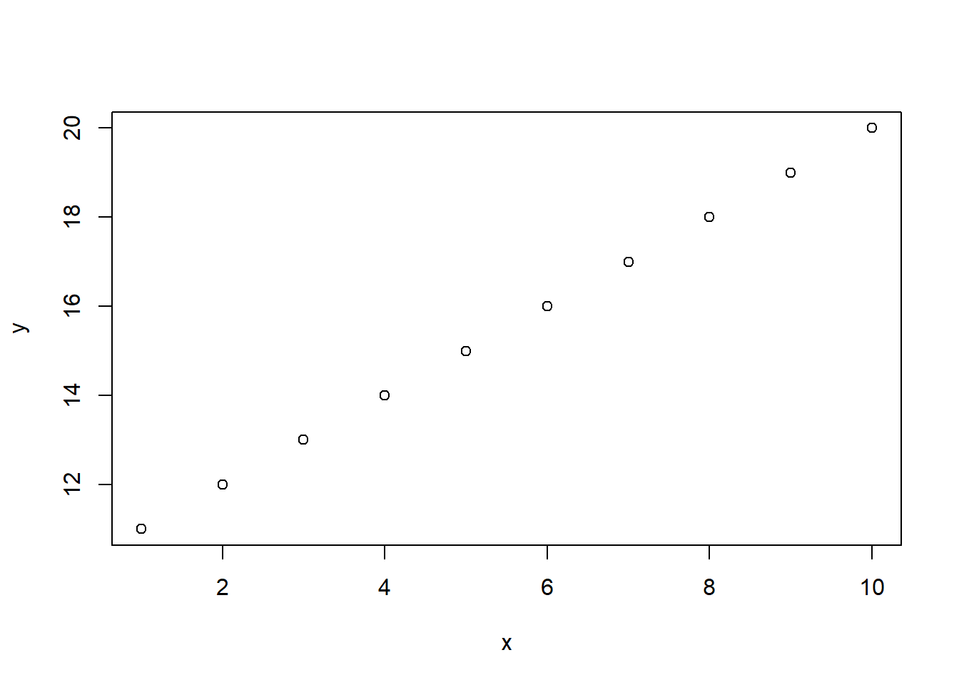
It is evident that it was very easy to create this plot. We simply
use the function plot() and include in the parentheses
our data frame. A scatterplot helps us visualize the data points
across two dimensions. For example, the first value of x is 1 and
the corresponding value of y is 11. This point is the one that
appears on the bottom left corner of the graph: there is a point
that is connected vertically to the value of 1 on the x axis and the
value of 11 in the y axis.
Before concluding this chapter, it is very important to discuss what
we would like to do when we need help regarding a function. It is
natural that sometimes we are not sure the arguments of a function,
and what kind of input is expected. Also, there could be times that
we forget the exact names of the arguments of a function. R provides
documentation of every function, which we can check
either by using a question mark (?), or by using the function
help(), in which we include the name of the function of
interest. For instance, suppose we want to check the documentation
of the function log(), a function that computes the
logarithm of a number. In that case, we use any one of the following
options to check its documentation:
# Help with question mark
?log

# Help with the function help()
help(log)
In both cases, the documentation appears in the bottom right panel, in the “Help” tab:

This is a very useful feature of R, and it works even without an internet connection. Since it’s common to forget the exact name of a function or its arguments, having this built-in support is especially helpful when learning new functions.
If we cannot recall at all the name of a function, we can utilize the search bar located in the “Help” pane. By typing key words related to the function we want, we should be able to locate it that way.